Debug Mode (in-situ visualization)

We have provided a mode that can display simulation results in real-time, which we call "debug mode." It is also backend-agnostic and happens to enable in-situ visualization. The original intent of this design was to allow users to immediately view the computation results while running a simulation. If the results do not develop as expected, the computation can be terminated at any time for a quick code review.

Note that this feature will only be enabled after the user explicitly calls WGLMakie:

using MaterialPointSolver
using WGLMakie

Note

• We implement this functionality through WGLMakie.jl, which theoretically supports computations on a remote headless server. However, as WGLMakie.jl is still in an experimental stage, we recommend launching Debug mode only on local machine for now.

• We prefer to always use the plot panel provided by the Julia Language plugin in VSCode to display results; please enable the plot panel in the julia-vscode plugin.

• The current maximum number of particles displayed is 500,000, but this can be customized by the user.

API

In normal mode, we assume that you have already instantiated and obtained args, grid, mp, attr, and bc.

materialpointsolver!(args, grid, mp, attr, bc)

where the type of debug is DebugConfig:

MaterialPointSolver.DebugConfig Type

DebugConfig

Description:

This struct is used to store the debug configurations for the in-situ visualization of the simulation.

• plot::DebugPlot : The WGLMakie configurations for the debug mode

• ... : More debug configurations can be added in the future

source

The current DebugPlot type has only one field, plot::DebugPlot, but more features may be added in the future.

The type of plot is DebugPlot:

MaterialPointSolver.DebugPlot Type

DebugPlot

Description:

This struct is used to store the WGLMakie configurations for the in-situ visualization of the simulation.

Users need to provice attr and cbname to specify the attribute to plot and the name of the colorbar, even you choose axis = false.

• axis::Bool = false : Whether to show the axis

• colorbar::Bool = true : Whether to show the colorbar

• colormap::Symbol = :readblue : The colormap for the plot

• pointsize::Real = 1f-2 : The size of the points

• pointnum::Int = 500000 : The number of points to plot

• tickformat::String = "{:9.2f}" : The format of the ticks

• calculate::Function = def_func : The function to calculate the value to plot

• axfontsize::Real = 24 : The font size of the axis

• cbfontsize::Real = 24 : The font size of the colorbar

• cbname::String : The name of the colorbar

source

Here, we may need to explain the meaning of the calculate field in DebugPlot. Sometimes, the values we want to display might be derived from multiple attributes, such as displacement, so we need to define the computation rules.

Note

• The return type of the user-defined calculate function must currently be a vector with the same length as the number of material points, and the input parameters of this custom function should always be: (i) grid, (ii) mp, (iii) attr, (iv) bc, and (v) vid, with the order fixed and unchangeable.

• Users can directly use debug=DebugConfig(), which will apply the default debug configuration, visualizing the color based on the density of the material points.

Examples

If you want to visualize the equivalent plastic strain, then：

plotfunc(grid, mp, attr, bc, vid) = Array{Float32, 1}(mp.ϵq)
plotconfig = DebugPlot(cbname="equivalent plastic strain", calculate=plotfunc)
debug = DebugConfig(plot=plotconfig)

DebugConfig(DebugPlot(false, true, :redblue, 0.01f0, 500000, "{:9.2f}", Main.plotfunc, 24, 24, "equivalent plastic strain"))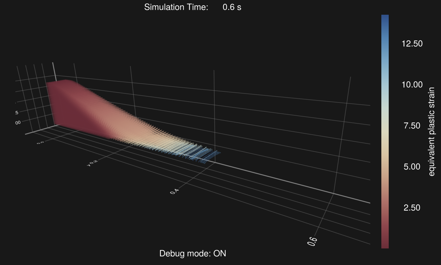

If you want to visualize the displacement：

function tmpf(grid, mp, attr, bc, vid)
    ξ0 = Array{Float32, 2}(mp.ξ0[vid, :])
    ξ1 = Array{Float32, 2}(mp.ξ[vid, :] )

    val = @. sqrt((ξ1[:, 1] - ξ0[:, 1])^2 .+
                  (ξ1[:, 2] - ξ0[:, 2])^2 .+
                  (ξ1[:, 3] - ξ0[:, 3])^2)
    return val
end
plotconfig = DebugPlot(pointsize=1, axis=true, axfontsize=10, calculate=tmpf, cbname="disp")
debug = DebugConfig(plotconfig)

DebugConfig(DebugPlot(true, true, :redblue, 1, 500000, "{:9.2f}", Main.tmpf, 10, 24, "disp"))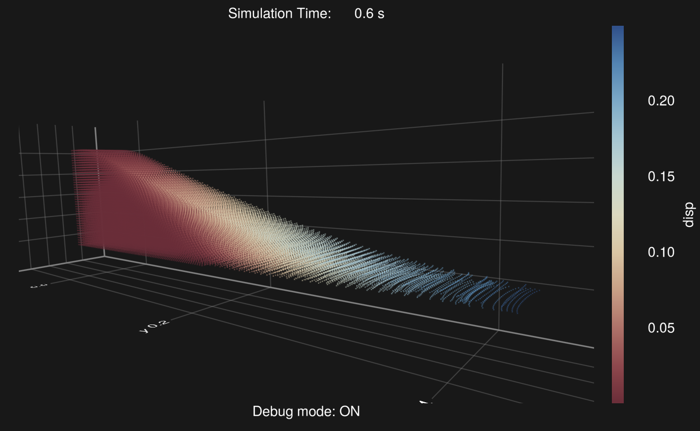

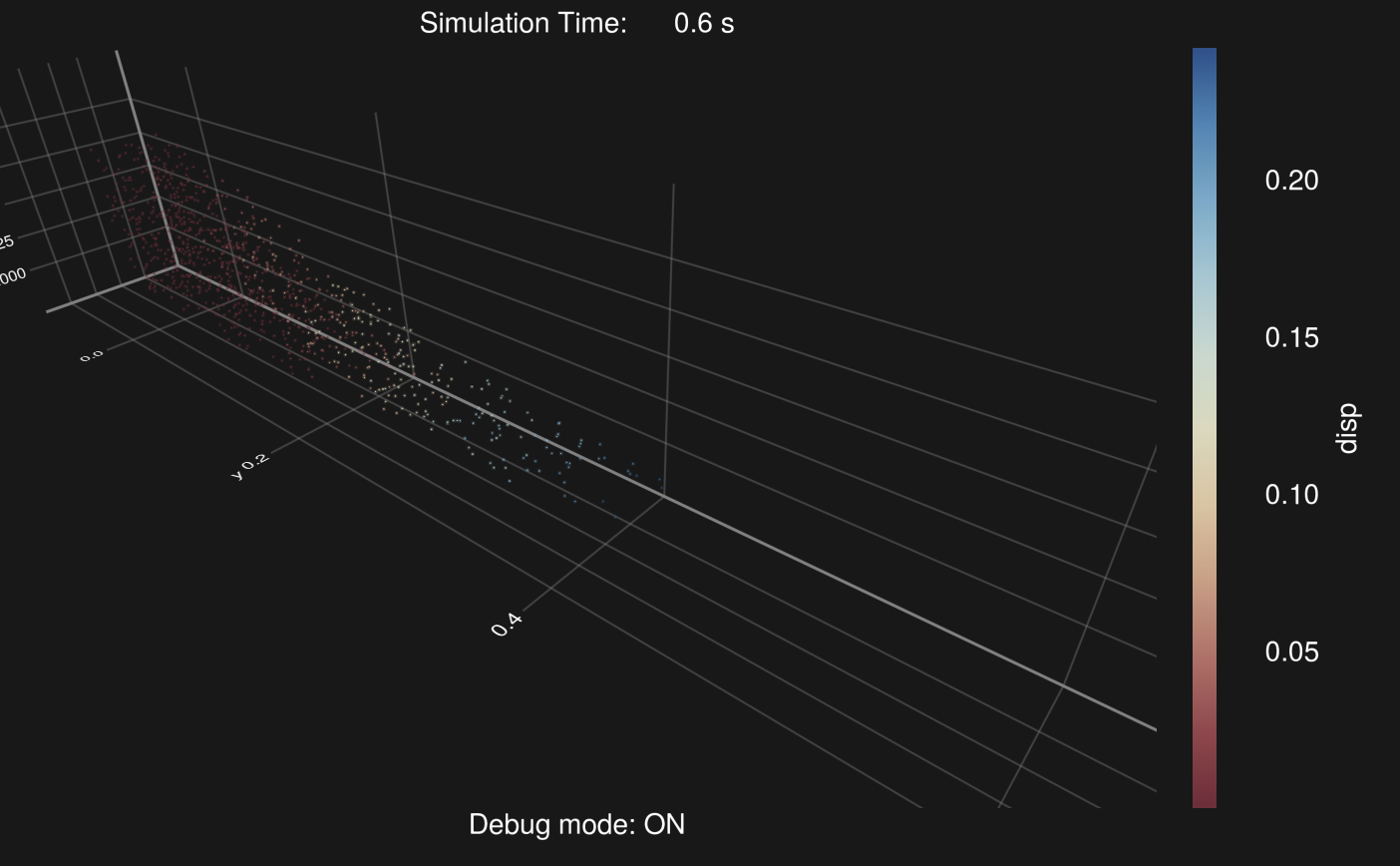
If you need a smooth visualization, try to decrease the pointsize or pointnum:

function tmpf(grid, mp, attr, bc, vid)
    ξ0 = Array{Float32, 2}(mp.ξ0[vid, :])
    ξ1 = Array{Float32, 2}(mp.ξ[vid, :] )

    val = @. sqrt((ξ1[:, 1] - ξ0[:, 1])^2 .+
                  (ξ1[:, 2] - ξ0[:, 2])^2 .+
                  (ξ1[:, 3] - ξ0[:, 3])^2)
    return val
end
plotconfig = DebugPlot(pointsize=1f-2, axis=true, axfontsize=10, calculate=tmpf, cbname="disp", pointnum=1000) 
debug = DebugConfig(plotconfig)

DebugConfig(DebugPlot(true, true, :redblue, 0.01f0, 1000, "{:9.2f}", Main.tmpf, 10, 24, "disp"))